What Is the Sharpe Ratio?
The Sharpe ratio compares the return of an investment with its risk. It’s a mathematical expression of the insight that excess returns over a period of time may signify more volatility and risk, rather than investing skill.1
Economist William F. Sharpe proposed the Sharpe ratio in 1966 as an outgrowth of his work on the capital asset pricing model (CAPM), calling it the reward-to-variability ratio.1 Sharpe won the Nobel Prize in economics for his work on CAPM in 1990.2
The Sharpe ratio’s numerator is the difference over time between realized, or expected, returns and a benchmark such as the risk-free rate of return or the performance of a particular investment category. Its denominator is the standard deviation of returns over the same period of time, a measure of volatility and risk.
Key Takeaways
- The Sharpe ratio divides a portfolio’s excess returns by a measure of its volatility to assess risk-adjusted performance
- Excess returns are those above an industry benchmark or the risk-free rate of return
- The calculation may be based on historical returns or forecasts
- A higher Sharpe ratio is better when comparing similar portfolios.
- The Sharpe ratio has inherent weaknesses and may be overstated for some investment strategies.
Formula and Calculation of Sharpe Ratio
In its simplest form,
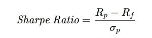
where:
Rp=return of portfolio
Rf=risk-free rate
σp=standard deviation of the portfolio’s excess return
Standard deviation is derived from the variability of returns for a series of time intervals adding up to the total performance sample under consideration.
The numerator’s total return differential versus a benchmark (Rp – Rf) is calculated as the average of the return differentials in each of the incremental time periods making up the total. For example, the numerator of a 10-year Sharpe ratio might be the average of 120 monthly return differentials for a fund versus an industry benchmark.
The Sharpe ratio’s denominator in that example will be those monthly returns’ standard deviation, calculated as follows:
- Take the return variance from the average return in each of the incremental periods, square it, and sum the squares from all of the incremental periods.
- Divide the sum by the number of incremental time periods.
- Take a square root of the quotient.
What the Sharpe Ratio Can Tell You
The Sharpe ratio is one of the most widely used methods for measuring risk-adjusted relative returns. It compares a fund’s historical or projected returns relative to an investment benchmark with the historical or expected variability of such returns.
The risk-free rate was initially used in the formula to denote an investor’s hypothetical minimal borrowing costs.1 More generally, it represents the risk premium of an investment versus a safe asset such as a Treasury bill or bond.
When benchmarked against the returns of an industry sector or investing strategy, the Sharpe ratio provides a measure of risk-adjusted performance not attributable to such affiliations.
The ratio is useful in determining to what degree excess historical returns were accompanied by excess volatility. While excess returns are measured in comparison with an investing benchmark, the standard deviation formula gauges volatility based on the variance of returns from their mean.
The ratio’s utility relies on the assumption that the historical record of relative risk-adjusted returns has at least some predictive value.1
Generally, the higher the Sharpe ratio, the more attractive the risk-adjusted return.
The Sharpe ratio can be used to evaluate a portfolio’s risk-adjusted performance. Alternatively, an investor could use a fund’s return objective to estimate its projected Sharpe ratio ex-ante.
The Sharpe ratio can help explain whether a portfolio’s excess returns are attributable to smart investment decisions or simply luck and risk.
For example, low-quality, highly speculative stocks can outperform blue chip shares for considerable periods of time, as during the Dot-Com Bubble or, more recently, the meme stocks frenzy. If a YouTuber happens to beat Warren Buffett in the market for a while as a result, the Sharpe ratio will provide a quick reality check by adjusting each manager’s performance for their portfolio’s volatility.
The greater a portfolio’s Sharpe ratio, the better its risk-adjusted performance. A negative Sharpe ratio means the risk-free or benchmark rate is greater than the portfolio’s historical or projected return, or else the portfolio’s return is expected to be negative.
:max_bytes(150000):strip_icc():format(webp)/william-f-sharpe_final-70794d182ddf4a26b92bed8c36f11a0b.png)
Sharpe Ratio Pitfalls
The Sharpe ratio can be manipulated by portfolio managers seeking to boost their apparent risk-adjusted returns history. This can be done by lengthening the return measurement intervals, which results in a lower estimate of volatility. For example, the standard deviation (volatility) of annual returns is generally lower than that of monthly returns, which are in turn less volatile than daily returns. Financial analysts typically consider the volatility of monthly returns when using the Sharpe ratio.
Calculating the Sharpe ratio for the most favorable stretch of performance rather than an objectively chosen look-back period is another way to cherry-pick the data that will distort the risk-adjusted returns.
The Sharpe ratio also has some inherent limitations. The standard deviation calculation in the ratio’s denominator, which serves as its proxy for portfolio risk, calculates volatility based on a normal distribution and is most useful in evaluating symmetrical probability distribution curves. In contrast, financial markets subject to herding behavior can go to extremes much more often than a normal distribution would suggest is possible. As a result, the standard deviation used to calculate the Sharpe ratio may understate tail risk.3
Market returns are also subject to serial correlation. The simplest example is that returns in adjacent time intervals may be correlated because they were influenced by the same market trend. But mean reversion also depends on serial correlation, just like market momentum. The upshot is that serial correlation tends to lower volatility, and as a result investment strategies dependent on serial correlation factors may exhibit misleadingly high Sharpe ratios as a result.4
One way to visualize these criticisms is to consider the investment strategy of picking up nickels in front of a steamroller that moves slowly and predictably nearly all the time, except for the few rare occasions when it suddenly and fatally accelerates. Because such unfortunate events are extremely uncommon, those picking up nickels would, most of the time, deliver positive returns with minimal volatility, earning high Sharpe ratios as a result. And if a fund picking up the proverbial nickels in front of a steamroller got flattened on one of those extremely rare and unfortunate occasions, its long-term Sharpe might still look good: just one bad month, after all. Unfortunately, that would bring little comfort to the fund’s investors.
Sharpe Alternatives: the Sortino and the Treynor
The standard deviation in the Sharpe ratio’s formula assumes that price movements in either direction are equally risky. In fact, the risk of an abnormally low return is very different from the possibility of an abnormally high one for most investors and analysts.
A variation of the Sharpe called the Sortino ratio ignores the above-average returns to focus solely on downside deviation as a better proxy for the risk of a fund of a portfolio.
The standard deviation in the denominator of a Sortino ratio measures the variance of negative returns or those below a chosen benchmark relative to the average of such returns.
Another variation of the Sharpe is the Treynor ratio, which divides excess return over a risk-free rate or benchmark by the beta of a security, fund, or portfolio as a measure of its systematic risk exposure. Beta measures the degree to which the volatility of a stock or fund correlates to that of the market as a whole. The goal of the Treynor ratio is to determine whether an investor is being compensated for extra risk above that posed by the market.
Example of How to Use Sharpe Ratio
The Sharpe ratio is sometimes used in assessing how adding an investment might affect the risk-adjusted returns of the portfolio.
For example, an investor is considering adding a hedge fund allocation to a portfolio that has returned 18% over the last year. The current risk-free rate is 3%, and the annualized standard deviation of the portfolio’s monthly returns was 12%, which gives it a one-year Sharpe ratio of 1.25, or (18 – 3) / 12.
The investor believes that adding the hedge fund to the portfolio will lower the expected return to 15% for the coming year, but also expects the portfolio’s volatility to drop to 8% as a result. The risk-free rate is expected to remain the same over the coming year.
Using the same formula with the estimated future numbers, the investor finds the portfolio would have a projected Sharpe ratio of 1.5, or (15% – 3%) divided by 8%.
In this case, while the hedge fund investment is expected to reduce the absolute return of the portfolio, based on its projected lower volatility it would improve the portfolio’s performance on a risk-adjusted basis. If the new investment lowered the Sharpe ratio it would be assumed to be detrimental to risk-adjusted returns, based on forecasts. This example assumes that the Sharpe ratio based on the portfolio’s historical performance can be fairly compared to that using the investor’s return and volatility assumptions.
What is a Good Sharpe Ratio?
Sharpe ratios above 1 are generally considered “good,” offering excess returns relative to volatility. However, investors often compare the Sharpe ratio of a portfolio or fund with those of its peers or market sector. So a portfolio with a Sharpe ratio of 1 might be found lacking if most rivals have ratios above 1.2, for example. A good Sharpe ratio in one context might be just a so-so one, or worse, in another.
How is the Sharpe Ratio Calculated?
To calculate the Sharpe ratio, investors first subtract the risk-free rate from the portfolio’s rate of return, often using U.S. Treasury bond yields as a proxy for the risk-free rate of return. Then, they divide the result by the standard deviation of the portfolio’s excess return.
Deep Understanding of the Sharpe Ratio
Since William Sharpe’s creation of the Sharpe ratio in 1966, it has been one of the most referenced risk/return measures used in finance, and much of this popularity is attributed to its simplicity.1 The ratio’s credibility was boosted further when Professor Sharpe won a Nobel Memorial Prize in Economic Sciences in 1990 for his work on the capital asset pricing model (CAPM).2
The Sharpe Ratio Defined
Most finance people understand how to calculate the Sharpe ratio and what it represents. The ratio describes how much excess return you receive for the extra volatility you endure for holding a riskier asset.3 Remember, you need compensation for the additional risk you take for not holding a risk-free asset.
We will give you a better understanding of how this ratio works, starting with its formula:
Return (rx)
The measured returns can be of any frequency (e.g., daily, weekly, monthly, or annually) if they are normally distributed. Herein lies the underlying weakness of the ratio: not all asset returns are normally distributed.
Kurtosis—fatter tails and higher peaks—or skewness can be problematic for the ratio as standard deviation is not as effective when these problems exist. Sometimes, it can be dangerous to use this formula when returns are not normally distributed.
Risk-Free Rate of Return (rf )
The risk-free rate of return is used to see if you are properly compensated for the additional risk assumed with the asset. Traditionally, the risk-free rate of return is the shortest-dated government T-bill (i.e. U.S. T-Bill). While this type of security has the least volatility, some argue that the risk-free security should match the duration of the comparable investment.
For example, equities are the longest duration asset available. Should they not be compared with the longest duration risk-free asset available: government-issued inflation-protected securities (IPS)? Using a long-dated IPS would certainly result in a different value for the ratio because, in a normal interest rate environment, IPS should have a higher real return than T-bills.
For instance, the Barclays Global Aggregate 10 Year Index returned 3.3% for the period ending Sept. 30, 2017, while the S&P 500 Index returned 7.4% within the same period.4 Some would argue that investors were fairly compensated for the risk of choosing equities over bonds. The bond index’s Sharpe ratio of 1.16% versus 0.38% for the equity index would indicate equities are the riskier asset.
Standard Deviation (StdDev(x))
Now that we have calculated the excess return by subtracting the risk-free rate of return from the return of the risky asset, we need to divide it by the standard deviation of the measured risky asset. As mentioned above, the higher the number, the better the investment looks from a risk/return perspective.
How the returns are distributed is the Achilles heel of the Sharpe ratio. Bell curves do not take big moves in the market into account. As Benoit Mandelbrot and Nassim Nicholas Taleb note in “How The Finance Gurus Get Risk All Wrong,” bell curves were adopted for mathematical convenience, not realism.5
However, unless the standard deviation is very large, leverage may not affect the ratio. Both the numerator (return) and denominator (standard deviation) could double with no problems. If the standard deviation gets too high, we see problems. For example, a stock that is leveraged 10-to-1 could easily see a price drop of 10%, which would translate to a 100% drop in the original capital and an early margin call.
The Sharpe Ratio and Risk
Understanding the relationship between the Sharpe ratio and risk often comes down to measuring the standard deviation, also known as the total risk. The square of standard deviation is the variance, which was widely used by Nobel Laureate Harry Markowitz, the pioneer of Modern Portfolio Theory.6
So why did Sharpe choose the standard deviation to adjust excess returns for risk, and why should we care? We know that Markowitz understood variance, a measure of statistical dispersion or an indication of how far away it is from the expected value, as something undesirable to investors.7 The square root of the variance, or standard deviation, has the same unit form as the analyzed data series and often measures risk.
The following example illustrates why investors should care about variance:
An investor has a choice of three portfolios, all with expected returns of 10% for the next 10 years. The average returns in the table below indicate the stated expectation. The returns achieved for the investment horizon is indicated by annualized returns, which takes compounding into account. As the data table and chart illustrates, the standard deviation takes returns away from the expected return. If there is no risk—zero standard deviation—your returns will equal your expected returns.
Expected Average Returns
| Year | Portfolio A | Portfolio B | Portfolio C |
| Year 1 | 10.00% | 9.00% | 2.00% |
| Year 2 | 10.00% | 15.00% | -2.00% |
| Year 3 | 10.00% | 23.00% | 18.00% |
| Year 4 | 10.00% | 10.00% | 12.00% |
| Year 5 | 10.00% | 11.00% | 15.00% |
| Year 6 | 10.00% | 8.00% | 2.00% |
| Year 7 | 10.00% | 7.00% | 7.00% |
| Year 8 | 10.00% | 6.00% | 21.00% |
| Year 9 | 10.00% | 6.00% | 8.00% |
| Year 10 | 10.00% | 5.00% | 17.00% |
| Average Returns | 10.00% | 10.00% | 10.00% |
| Annualized Returns | 10.00% | 9.88% | 9.75% |
| Standard Deviation | 0.00% | 5.44% | 7.80% |
Using the Sharpe Ratio
The Sharpe ratio is a measure of return often used to compare the performance of investment managers by making an adjustment for risk.
For example, Investment Manager A generates a return of 15%, and Investment Manager B generates a return of 12%. It appears that manager A is a better performer. However, if manager A took larger risks than manager B, it may be that manager B has a better risk-adjusted return.
To continue with the example, say that the risk-free rate is 5%, and manager A’s portfolio has a standard deviation of 8% while manager B’s portfolio has a standard deviation of 5%. The Sharpe ratio for manager A would be 1.25, while manager B’s ratio would be 1.4, which is better than that of manager A. Based on these calculations, manager B was able to generate a higher return on a risk-adjusted basis.
For some insight, a ratio of 1 or better is good, 2 or better is very good, and 3 or better is excellent.
The Bottom Line
Risk and reward must be evaluated together when considering investment choices; this is the focal point presented in Modern Portfolio Theory.7 In a common definition of risk, the standard deviation or variance takes rewards away from the investor. As such, always address the risk along with the reward when choosing investments. The Sharpe ratio can help you determine the investment choice that will deliver the highest returns while considering risk.